Experimental variogram
Overview
The experimental variogram calculation is adapted from geostatsmodels to handle both 2D and 3D cases. Results are checked against Isatis for sanity (see unit tests).
Algorithm
Compute 3D distances pairwaise between points in dataset
Identify pairs of points included in a lag range
Given azimuth, dip and pitch angle inputs, identify pairs belonging to an angular range (considering an input angular tolerance). Matching pairs are also selected at opposite angle (180° azimuth rotation)
The semivariance (or covariogram, depending on user’s choice) is then computed for all the lags, according to the input values of each points for all the selected pairs.
Input
The variogram calculations accepts the following angles in degrees:
azimuth: clockwise angle from the North on the horizontal plane, giving the strike direction
dip: angle from horizontal plane along the dipping direction (perpendicular to the strike direction)
pitch: clockwise angle from the strike direction on the dipping plane
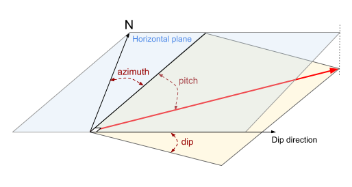
A 3D interactive tool is available to help you visualize these angles.
Angular tolerance (atol) in degrees, slicing width and slicing
height are defined as below: 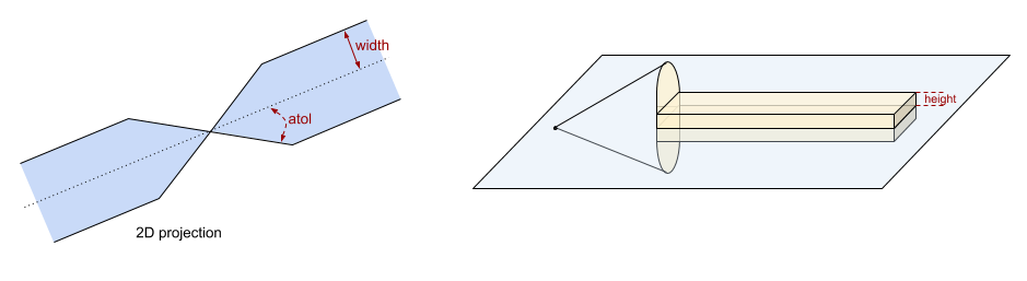
Output
The geolime variogram output is intended to be as close as Isatis output. A typical geolime variogram outputs:
rank npairs  lag  avgdist        vario
0     4      1   60  57.6806  1568.000000
1     5      3   75  71.9403  2608.166667
2     6      2   90  86.3444   759.250000
3     7      1  105  105.894    32.000000
4     8      2  120  122.254   740.000000
5     9      2  135  130.186  5870.250000
6    10      2  150  151.782   900.250000
7    11      2  165  170.897  2866.250000
8    12      2  180  185.647  2358.250000
9    13      4  195  198.692   345.625000
10   14     10  210  211.139  1274.000000